Before we start today’s section, we ask that you complete the course evaluations for
this class. The evaluations can be found here. These submissions are anonymous,
so please answer honestly about the course, Dr. Sullivan, and your TAs.
Graphs
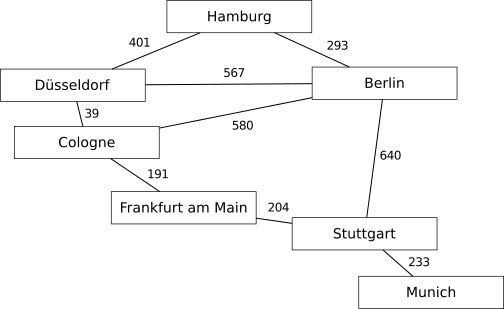
Consider the following weighted, undirected graph representing the
distances from city to city by way of the Autobahn in Germany.
Is this graph acyclic? If the graph is cyclic, provide an
example of a cycle. 4
If we used an adjacency matrix to represent this graph,
what would it look like? Assume that the vertices are numbered
alphabetically, starting from zero. 5
Graph traversals
For the following graph traversals, list the order in which the cities
would be considered and draw the resulting spanning tree.
Perform a depth-first traversal of the graph, starting
from Düsseldorf. List the order in which cities are considered and
draw the resulting spanning tree. 6
Perform a breadth-first traversal of the graph, starting
from Berlin. List the order in which cities are considered and
draw the resulting spanning tree. 7
Minimum spanning trees
Use Prim’s minimum spanning tree algorithm to obtain a minimum-cost
spanning tree from the graph. Start by adding Hamburg to the singleton
set. Then list the edges added to the tree as the algorithm runs, and
draw the resulting tree. 8
Finding shortest paths
Use Dijkstra’s shortest path algorithm to obtain the shortest paths
starting from Cologne. 9
Berlin’s neighbors are Hamburg, Düsseldorf, Cologne, and Stuttgart. ↩
This graph is connected, since there is a path from one vertex to any
other vertex in the graph. ↩
This graph is not complete, since there is not an edge from each
vertex to every other vertex in the graph. ↩
This graph has at least one cycle. It is therefore cyclic, or
not acyclic. An example of a cycle is the one formed among
Hamburg, Berlin, and Düsseldorf. ↩
Here’s the adjacency matrix. Each vertex is labeled with the first
letter of its name.
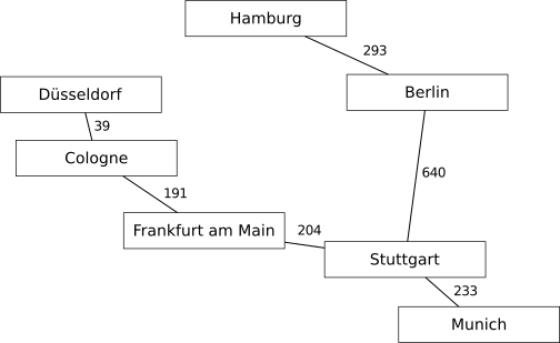
A depth-first traversal from Düsseldorf results in the following sequence of
visited vertices: Düsseldorf, Cologne, Frankfurt am Main, Stuttgart, Munich,
Berlin, Hamburg. Here’s the spanning tree:
The spanning tree obtained from depth-first search.
↩
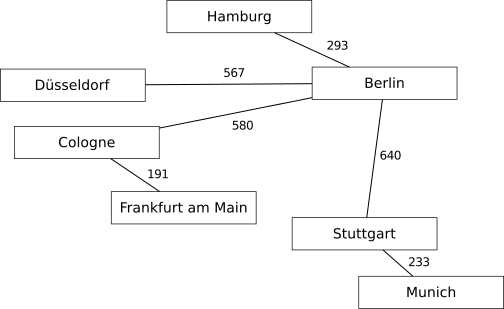
A breadth-first traversal from Berlin results in the following sequence of
visited vertices: Berlin, Hamburg, Düsseldorf, Cologne, Stuttgart,
Frankfurt, Munich.
The spanning tree obtained from breadth-first search.
↩
Here’s the table showing the edges added to set A from set B,
where A initially contains Hamburg. Each city is denoted by
the first letter in its name.